Hanborq Improved Hadoop MapReduce

Open Source: https://github.com/hanborq/hadoop

Major Features:

1. Worker Pool

Does not spawn new JVM processes for each job/task, but instead start these slot/worker processes at initialization phase and keep them running constantly.

2. Sort Avoidance.

Many aggregation job need not sort.

---------------------

A Hanborq optimized Hadoop Distribution, especially with high performance of MapReduce. It's the core part of HDH (Hanborq Distribution with Hadoop for Big Data Engineering).

Here is our presentation: Hanborq Optimizations on Hadoop MapReduce

Hanborq optimizations on hadoop map reduce 20120221a

HDH (Hanborq Distribution with Hadoop)

Hanborq, a start-up team focuses on Cloud & BigData products and businesses, delivers a series of software products for Big Data Engineering, including a optimized Hadoop Distribution.

HDH delivers a series of improvements on Hadoop Core, and Hadoop-based tools and applications for putting Hadoop to work solving Big Data problems in production. HDH is ideal for enterprises seeking an integrated, fast, simple, and robust Hadoop Distribution. In particular, if you think your MapReduce jobs are slow and low performing, the HDH may be you choice.

Hanborq optimized Hadoop

It is a open source distribution, to make Hadoop Fast, Simple and Robust.
- Fast: High performance, fast MapReduce job execution, low latency.
- Simple: Easy to use and develop BigData applications on Hadoop.
- Robust: Make hadoop more stable.

MapReduce Benchmarks

The Testbed: 5 node cluster (4 slaves), 8 map slots and 2 reduce slots per node.

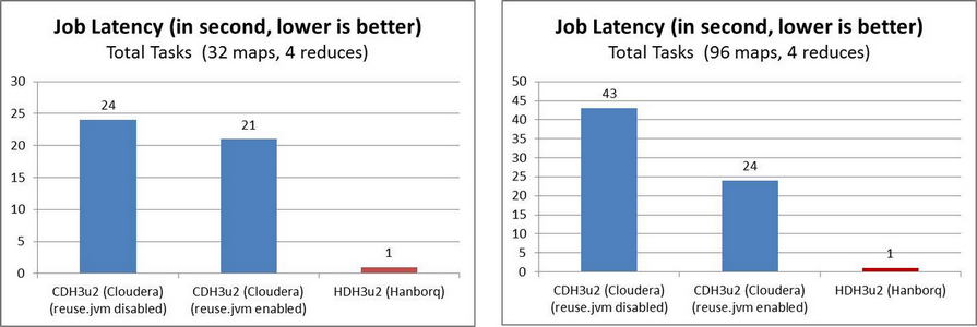
1. MapReduce Runtime Environment Improvement
In order to reduce job latency, HDH implements Distributed Worker Pool like Google Tenzing. HDH MapReduce framework does not spawn new JVM processes for each job/task, but instead keep the slot processes running constantly. Additionally, there are many other improvements at this aspect.
bin/hadoop jar hadoop-examples-0.20.2-hdh3u3.jar sleep -m 32 -r 4 -mt 1 -rt 1
bin/hadoop jar hadoop-examples-0.20.2-hdh3u3.jar sleep -m 96 -r 4 -mt 1 -rt 1

2. MapReduce Processing Engine Improvement
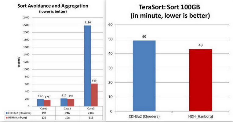
Many improvements are applied on Hadoop MapReduce Processing engine, such as shuffle, sort-avoidance, etc. 

Please refer to the page MapReduce Benchmarks for detail.

Features

MapReduce

- Fast job launching: such as the time of job lunching drop from 20 seconds to 1 second.
- Low latency: not only job setup, job cleanup, but also data shuffle, etc.
- High performance shuffle: low overhead of CPU, network, memory, disk, etc.
- Sort avoidance: some case of jobs need not sorting, which result in too many unnecessary system overhead and long latency.

... and more and continuous ...

How to build?

$ cd cloudera/maven-packaging  
$ mvn -Dnot.cdh.release.build=true -Dmaven.test.skip=true -DskipTests=true clean package  

Then use this package: build/hadoop-{main-version}-hdh{hdh-version}, for example: build/hadoop-0.20.2-hdh3u2

Compatibility

The API, configuration, scripts are all back-compatible with Apache Hadoop and Cloudera Hadoop(CDH). The user and developer need not to study new, except new features.

Innovations and Inspirations

The open source community and our real enterprise businesses are the strong source of our continuous innovations. Google, the great father of MapReduce, GFS, etc., always outputs papers and experiences that bring us inspirations, such as:
MapReduce: Simplified Data Processing on Large Clusters
MapReduce: A Flexible Data Processing Tool
Tenzing: A SQL Implementation On The MapReduce Framework
Dremel: Interactive Analysis of Web-Scale Datasets

... and more and more ...

Open Source License

All Hanborq offered code is licensed under the Apache License, Version 2.0. And others follow the original license announcement.

Hadoop is a tool that still needs work.

Cloudera wants to tackle Hadoop the way RedHat tackled Linux - offer support, services, and additional around it. I think it may be too early, it may be the reason why Bisciglia(Wibidata,Ex-googler) and Srivas(MapR,Ex-googler) left Cloudera.

Maybe Googlers know clearer of the gaps.

http://www.wired.com/wiredenterprise/2011/12/ex-google-man/ 

The Integration of Analytic DBMS and Hadoop

Recently, tow famous vendors of analytic DBMS, Vertica and Aster-Data announced their integration with Hadoop. The analytic DBMS and Hadoop, each address distinct but complementary problems for managing large data.

Vertica:

Currently it is a light integration.

• ETL, ELT, data cleansing, data mining, etc.
• Moving data between Hadoop and Vertica.
• InputFormat (InputSplit , VerticaRecord, push down relational map operations by parameterizing the database query).
• OutputFormat (to existing or create a new table).
• Easy for Hadoop developers to push down Map operations to Vertica databases in parallel by specifying parameterized queries which result in pre-aggregated data for each mapper.
• Support Hadoop streaming interface.

Typical usages:
(1) Raw Data->Hadoop(ETL)->Vertical (for fast ad-hoc query, near realtime)
(2) Vertical -> Hadoop(ETL) ->Vertical (for fast ad-hoc query, near realtime)
(3) Vertical -> Hadoop (sophisticated query for analysis or mining)

We can expect to see tighter integration and higher performance.

References
[1] The Scoop on Hadoop and Vertica: http://databasecolumn.vertica.com/2009/09/the_scoop_on_hadoop_and_vertic.html
[2] Using Vertica as a Structured Data Repository for Apache Hadoop: http://www.vertica.com/MapReduce
[3] Cloudera DBInputFormat interface: http://www.cloudera.com/blog/2009/03/06/database-access-with-hadoop/
[4] Managing Big Data with Hadoop and Vertica: http://www.vertica.com/resourcelogin?type=pdf&item=ManagingBigDatawithHadoopandVertica.pdf

AsterData:

AsterData already provide in-database MapReduce.

The new Aster-Hadoop Data Connector, which utilizes Aster’s patent-pending SQL-MapReduce capabilities for two-way, high-speed, data transfer between Apache Hadoop and Aster Data’s massively parallel data warehouse.

• ETL processing or data mining, and then pull that data into Aster for interactive queries or ad-hoc analytics on massive data scales.
• The Connector utilizes key new SQL-MapReduce functions to provide ultra-fast, two-way data loading between HDFS (Hadoop Distributed File System) and Aster Data’s MPP Database.
• Parallel loader.
• LoadFromHadoop: Parallel data loading from HDFS to Aster nCluster.
• LoadToHadoop: Parallel data loading from Aster nCluster to HDFS.

Key advantages of Aster’s Hadoop Connector include:

• High-performance: Fast, parallel data transfer between Hadoop and Aster nCluster.
• Ease-of-use: Analysts can now seamlessly invoke a SQL command for ultra-simple import of Hadoop-MapReduce jobs, for deeper data analysis. Aster intelligently and automatically parallelizes the load.
• Data Consistency: Aster Data's data integrity and transactional consistency capabilities treat the data load as a 'transaction', ensuring that the data load or export is always consistent and can be carried out while other queries are running in parallel in Aster.
• Extensibility: Customers can easily further extend the Connector using SQL-MapReduce, to provide further customization for their specific environment.

The typical usages are similar to Vertica.

References
[1] Aster Data Announces Seamless Connectivity With Hadoop: http://www.nearshorejournal.com/2009/10/aster-data-announces-seamless-connectivity-with-hadoop/
http://www.asterdata.com/news/091001-Aster-Hadoop-connector.php
[2] DBMS2 - MapReduce tidbits http://www.dbms2.com/2009/10/01/mapreduce-tidbits/#more-983
[3] AstaData Blog: Aster Data Seamlessly Connects to Hadoop, http://www.asterdata.com/blog/index.php/2009/10/05/aster-data-seamlessly-connects-to-hadoop/

Another Integration of Analytic DBMS and Hadoop case is HadoopDB project. http://db.cs.yale.edu/hadoopdb/hadoopdb.html

Tips of Hadoop Runtime Environment

To setup a cluster for running Hadoop/HBase/Hive, etc., besides the configuration and tuning of these open-source programs themselves, the system hardware and software, and some useful utilities, should also be considered to improve the system performance and to ease the system maintenance.

1. Cluster Facilities and Hardware [1]

(1) Data center:

Usually, we run Hadoop/HBase/Hive in a single data center.

(2) Servers:

Clusters are often either capacity bound or CPU bound.

The 1U or 2U configuration is usually used.

The storage capability of each node is usually not too dense (<= 4TB is recommended).

Commodity server: 2x4 core CPU, 16 GB RAM, 4x1TB SATA, 2x1 GE NIC

Use ECC RAM and cheap hard drives: 7200 RPM SATA.

Start with standard 64-bit box for masters and workers.

(3) Network:

Gigabit Ethernet, 2 level tree, 5:1 oversubscription to core

May want redundancy at top of rack and core

Usually, for a small cluster, all nodes are under a single GE switch.

(4) RAID configuration: RAID0

If there are two or more disks in each machine, RAID0 can provide better disk throughput than other RAID levels (and JBOD?). The multiple data replicas of HDFS can tolerate failure and guarantee the data safety.

2. System Software

(1) Linux:

RedHat5+ or CentOS5+ (recommended). Now, we use CentOS5.3-x64.

(2) Local File System:

Ext3 is ok.

We usually configure a separate disk partition for Hadoop used local file system, create and mount separate local file system for Hadoop.

Mount with noatime and nodiratime for performance improvements. Default, Linux will update the atime of files and directories, which is unnecessary in most cases. [2]

-- Edit /etc/fstab:

e.g. /dev/VolGroup00/LogVol02 /data ext3 defaults,noatime,nodiratime 1 2

-- remound:

mount -o remount /data

(3) Swappiness configuration: [3]

With the introduction of version 2.6, the new variable "swappiness" was added in the Linux kernel memory management subsystem and a tunable was created for it. High value of swappiness will make the kernel page out application text in favour of another application or even file-system cache. The default value is 60 (see mm/vmscan.c).

If you end up swapping, you're going to start seeing some weird behavior and very slow GC runs, and likely killing off HBase regionservers as ZooKeeper times out and assume the RegionServer is dead. Suggest setting vm.swappiness = 0 or other low number (e.g. 10), and observe the state of swap.

-- Edit /etc/sysctl.conf : vm.swappiness=0

-- To check the current value on a running system: sysctl vm.swappiness

(4) Linux default file handle limit: [4]

Currently HBase is a file handle glutton. To up the users' file handles, edit /etc/security/limits.conf on all nodes.

* - nofile 32768

(5) Java: JRE/JDK1.6 latest and GC options [5]

For machine with 4-16 cores, our Hadoop/HBase and other java applications should use GC option as: “-XX:+UseConcMarkSweepGC”.

For machine with 2 cores, should use GC option as: “-XX:+UseConcMarkSweepGC -XX:+CMSIncrementalMode”.

(6) Apache ANT 1.7.1

(7) Useful Linux utilities:

top, sar, iostat, iftop, vmstat, nfsstat, strace, dmesg, and friends

Especially iostat is very useful for disk I/O analysis.

(8) Useful java utilities:

jps, jstack, jconsole

(9) Compression native library: Gzip and LZO [7]

(10) Ganglia:

To integrate metrics of Hadoop, HBase, Hive, applications, and Linux system.

References:

[1] Hadoop and Cloudera, Managing Petabytes with Open Source, Jeff Hammerbacher, Aug. 21 http://indico.cern.ch/conferenceDisplay.py?confId=59791 or http://bit.ly/NXH6p

[2] Set noatime of local file system: http://www.chinaz.com/Server/Linux/0515L0032009.html

[3] Linux Swappiness: http://www.sollers.ca/blog/2008/swappiness/

[4] HBase FAQ: http://wiki.apache.org/hadoop/Hbase/FAQ

[5] Java SE 6 HotSpot[tm] Virtual Machine Garbage Collection Tuning, http://java.sun.com/javase/technologies/hotspot/gc/gc_tuning_6.html

[6] Apache Ant: http://ant.apache.org/

[7] http://cloudepr.blogspot.com/2009/09/hfile-block-indexed-file-format-to.html

HFile: A Block-Indexed File Format to Store Sorted Key-Value Pairs

1. Intruduction

HFile is a mimic of Google’s SSTable. Now, it is available in Hadoop HBase-0.20.0. And the previous releases of HBase temporarily use an alternate file format – MapFile[4], which is a common file format in Hadoop IO package. I think HFile should also become a common file format when it becomes mature, and should be moved into the common IO package of Hadoop in the future.

Following words of SSTable are from section 4 of Google’s Bigtable paper.

The Google SSTable file format is used internally to store Bigtable data. An SSTable provides a persistent, ordered immutable map from keys to values, where both keys and values are arbitrary byte strings. Operations are provided to look up the value associated with a specified key, and to iterate over all key/value pairs in a specified key range. Internally, each SSTable contains a sequence of blocks (typically each block is 64KB in size, but this is configurable). A block index (stored at the end of the SSTable) is used to locate blocks; the index is loaded into memory when the SSTable is opened. A lookup can be performed with a single disk seek: we first find the appropriate block by performing a binary search in the in-memory index, and then reading the appropriate block from disk. Optionally, an SSTable can be completely mapped into memory, which allows us to perform lookups and scans without touching disk.[1]

The HFile implements the same features as SSTable, but may provide more or less.

2. File Format

Data Block Size

Whenever we say Block Size, it means the uncompressed size.

The size of each data block is 64KB by default, and is configurable in HFile.Writer. It means the data block will not exceed this size more than one key/value pair. The HFile.Writer starts a new data block to add key/value pairs if the current writing block is equal to or bigger than this size. The 64KB size is same as Google’s [1].

To achieve better performance, we should select different block size. If the average key/value size is very short (e.g. 100 bytes), we should select small blocks (e.g. 16KB) to avoid too many key/value pairs in each block, which will increase the latency of in-block seek, because the seeking operation always finds the key from the first key/value pair in sequence within a block.

Maximum Key Length

The key of each key/value pair is currently up to 64KB in size. Usually, 10-100 bytes is a typical size for most of our applications. Even in the data model of HBase, the key (rowkey+column family:qualifier+timestamp) should not be too long.

Maximum File Size

The trailer, file-info and total data block indexes (optionally, may add meta block indexes) will be in memory when writing and reading of an HFile. So, a larger HFile (with more data blocks) requires more memory. For example, a 1GB uncompressed HFile would have about 15600 (1GB/64KB) data blocks, and correspondingly about 15600 indexes. Suppose the average key size is 64 bytes, then we need about 1.2MB RAM (15600X80) to hold these indexes in memory.

Compression Algorithm

- Compression reduces the number of bytes written to/read from HDFS.

- Compression effectively improves the efficiency of network bandwidth and disk space

- Compression reduces the size of data needed to be read when issuing a read

To be as low friction as necessary, a real-time compression library is preferred. Currently, HFile supports following three algorithms:

(1)NONE (Default, uncompressed, string name=”none”)

(2)GZ (Gzip, string name=”gz”)

Out of the box, HFile ships with only Gzip compression, which is fairly slow.

(3)LZO(Lempel-Ziv-Oberhumer, preferred, string name=”lzo”)

To achieve maximal performance and benefit, you must enable LZO, which is a lossless data compression algorithm that is focused on decompression speed.

Following figures show the format of an HFile.

In above figures, an HFile is separated into multiple segments, from beginning to end, they are:

- Data Block segment

To store key/value pairs, may be compressed.

- Meta Block segment (Optional)

To store user defined large metadata, may be compressed.

- File Info segment

It is a small metadata of the HFile, without compression. User can add user defined small metadata (name/value) here.

- Data Block Index segment

Indexes the data block offset in the HFile. The key of each index is the key of first key/value pair in the block.

- Meta Block Index segment (Optional)

Indexes the meta block offset in the HFile. The key of each index is the user defined unique name of the meta block.

- Trailer

The fix sized metadata. To hold the offset of each segment, etc. To read an HFile, we should always read the Trailer firstly.

The current implementation of HFile does not include Bloom Filter, which should be added in the future.

3. LZO Compression

LZO is now removed from Hadoop or HBase 0.20+ because of GPL restrictions. To enable it, we should install native library firstly as following. [6][7][8][9]

(1) Download LZO: http://www.oberhumer.com/, and build.

# ./configure --build=x86_64-redhat-linux-gnu --enable-shared --disable-asm

# make

# make install

Then the libraries have been installed in: /usr/local/lib

(2) Download the native connector library http://code.google.com/p/hadoop-gpl-compression/, and build.

Copy hadoo-0.20.0-core.jar to ./lib.

# ant compile-native

# ant jar

(3) Copy the native library (build/native/ Linux-amd64-64) and hadoop-gpl-compression-0.1.0-dev.jar to your application’s lib directory. If your application is a MapReduce job, copy them to hadoop’s lib directory. Your application should follow the $HADOOP_HOME/bin/hadoop script to ensure that the native hadoop library is on the library path via the system property -Djava.library.path=. [9]

4. Performance Evaluation

Testbed

− 4 slaves + 1 master

− Machine: 4 CPU cores (2.0G), 2x500GB 7200RPM SATA disks, 8GB RAM.

− Linux: RedHat 5.1 (2.6.18-53.el5), ext3, no RAID, noatime

− 1Gbps network, all nodes under the same switch.

− Hadoop-0.20.0 (1GB heap), lzo-2.0.3

Some MapReduce-based benchmarks are designed to evaluate the performance of operations to HFiles, in parallel.

− Total key/value entries: 30,000,000.

− Key/Value size: 1000 bytes (10 for key, and 990 for value). We have totally 30GB of data.

− Sequential key ranges: 60, i.e. each range have 500,000 entries.

− Use default block size.

− The entry value is a string, each continuous 8 bytes are a filled with a same letter (A~Z). E.g. “BBBBBBBBXXXXXXXXGGGGGGGG……”.

We set mapred.tasktracker.map.tasks.maximum=3 to avoid client side bottleneck.

(1) Write

Each MapTask for each range of key, which writes a separate HFile with 500,000 key/value entries.

(2) Full Scan

Each MapTask scans a separate HFile from beginning to end.

(3) Random Seek a specified key

Each MapTask opens one separate HFile, and selects a random key within that file to seek it. Each MapTask runs 50,000 (1/10 of the entries) random seeks.

(4) Random Short Scan

Each MapTask opens one separate HFile, and selects a random key within that file as a beginning to scan 30 entries. Each MapTask runs 50,000 scans, i.e. scans 50,000*30=1,500,000 entries.

This table shows the average entries which are written/seek/scanned per second, and per node.

In this evaluation case, the compression ratio is about 7:1 for gz(Gzip), and about 4:1 for lzo. Even through the compression ratio is just moderate, the lzo column shows the best performance, especially for writes.

The performance of full scan is much better than SequenceFile, so HFile may provide better performance to MapReduce-based analytical applications.

The random seek in HFiles is slow, especially in none-compressed HFiles. But the above numbers already show 6X~10X better performance than a disk seek (10ms). Following Ganglia charts show us the overhead of load, CPU, and network. The random short scan makes the similar phenomena.

HFile: A Block-Indexed File Format to Store Sorted Key-Value Pairs

View more documents from schubertzhang.

References

[1] Google, Bigtable: A Distributed Storage System for Structured Data, http://labs.google.com/papers/bigtable.html

[2] HBase-0.20.0 Documentation, http://hadoop.apache.org/hbase/docs/r0.20.0/

[3] HFile code review and refinement. http://issues.apache.org/jira/browse/HBASE-1818

[4] MapFile API: http://hadoop.apache.org/common/docs/current/api/org/apache/hadoop/io/MapFile.html

[5] Parallel LZO: Splittable Compression for Hadoop. http://www.cloudera.com/blog/2009/06/24/parallel-lzo-splittable-compression-for-hadoop/

http://blog.chrisgoffinet.com/2009/06/parallel-lzo-splittable-on-hadoop-using-cloudera/

[6] Using LZO in Hadoop and HBase: http://wiki.apache.org/hadoop/UsingLzoCompression

[7] LZO: http://www.oberhumer.com

[8] Hadoop LZO native connector library: http://code.google.com/p/hadoop-gpl-compression/

[9] Hadoop Native Libraries Guide: http://hadoop.apache.org/common/docs/r0.20.0/native_libraries.html